Chapter 11 Exporting Results

After the analysis, export the results from the Export split button at the bottom right of the central plot area. Save numerical data with Export results (CSV), plot images with Export images (PNG), and reports with Export report (PDF) or Export report (Word).

On macOS, double-clicking a ZIP extracts it in the same location.

Important: The Free Energy and Model Posterior Probability recorded in exports cannot be compared across the Height / Area intensity parametrizations. Comparisons are valid only within a run using the same parametrization.

11.1 Export Menu

Pressing the arrow of the split button opens a menu for choosing the export format.

Menu	Output file	Contents
Export results (CSV)	<timestamp>-<dataset>_results.zip	Numerical data for all models, analysis settings, model comparison
Export images (PNG)	<timestamp>-<dataset>_images.zip	Plot images for all models and a manifest
Export report (PDF)	<timestamp>-<dataset>_report.pdf	PDF report
Export report (Word)	<timestamp>-<dataset>_report.docx	Word report
Advanced…	Per settings	Select CSV / Charts / Report

<timestamp> is the analysis completion time in JST in the YYYY-MM-DDTHH-mm-ss format. <dataset> is the dataset name. For the regular PDF / Word exports, the default suffix _report is appended to the file name. If you change the suffix in Advanced Export, that suffix is inserted just before the extension of the PDF / Word report file name (it is not appended to ZIP file names).

Inline edits of axis labels, inline edits of legend labels, and legend show / hide are also used for image and report outputs. The other Plot Settings (font size, markers, line styles) are for on-screen display only and are not reflected in outputs.

11.2 Structure of <timestamp>-<dataset>_results.zip

<timestamp>-<dataset>_results/
├── summary.json
├── experiment_config.json
├── model_comparison.csv
├── Gaussian-8peaks/
├── Gaussian-9peaks/
├── Gaussian-10peaks/
├── pseudoVoigt-8peaks/
├── pseudoVoigt-9peaks/
└── pseudoVoigt-10peaks/

Subfolder names follow <basisFunc>-<peakCount>peaks/. For example, Gaussian models are output as Gaussian-10peaks/, Lorentzian models as Lorentzian-10peaks/, and pseudo-Voigt models as pseudoVoigt-10peaks/.

Files Directly Under the Root

File	Contents
summary.json	Dataset name, date and time, number of data points, X/Y axes, best model information. For Area results, the parametrization / Area prior / constraint provenance are also recorded
experiment_config.json	Basis function, Noise settings, Offset settings, Global prior ranges, Sampling settings. For Area results, the Area-native settings are recorded
model_comparison.csv	Free Energy, Posterior Probability, and Best / Selected flags for each model

For Height results, model_comparison.csv remains Model, Free_Energy, Posterior_Probability, Is_Best_Model, Is_Selected_Model as before. Only for Area results, an Intensity_Parametrization column is added immediately after Model, with the value Area. The Model column uses the pseudoVoigt-10peaks format, and the flag columns are Yes / No.

Area results record the intensity parametrization, Area prior, constraints, shape-link settings, and other information needed to interpret the result. Output column names follow the corresponding Height or Area export format. The pseudo-Voigt mixing ratio is exported as MixRatio_Area (\(\eta_A\)) for Area results and as the legacy MixRatio (\(\eta_H\)) for Height results.

The peak-count search range, per-peak priors from Set per peak, and fixed Noise values are not included, so if you need a complete record of the analysis conditions, also record the values from the settings screen separately.

When a Reference offset was used, experiment_config.json stores the selected reference name, the source file of the reference, the X/Y columns used for the reference, and the number of points. The PDF report also records the selected reference name and its source file.

11.3 Structure of the Per-Model Subfolders

Each subfolder contains the files corresponding to that model.

<basisFunc>-<peakCount>peaks/
├── fit_curve.csv
├── parameter_summary.csv
├── posterior_samples.csv
├── statistics.json
└── energy_trace.csv

File	Contents
fit_curve.csv	Observed X/Y spectrum, each peak curve, Offset_Fit, Combined_Fit
parameter_summary.csv	MAP estimates and 95% credible intervals
posterior_samples.csv	Posterior distribution samples. When large, they are thinned for output
statistics.json	Analysis summary including peak_count, total_samples, free_energy, and posterior_probability
energy_trace.csv	Energy trace of the sampling process. Output by the CPU version only; not output by the GPU version

Depending on the result format, histogram_*.csv may be output instead of posterior_samples.csv. For Area results the intensity distribution is histogram_Area.csv and the pseudo-Voigt \(\eta_A\) is histogram_MixRatio_Area.csv; Height results keep histogram_Height.csv / histogram_MixRatio.csv. CPU results may also include noise_parameters.csv.

11.4 Columns of fit_curve.csv

fit_curve.csv uses the fixed column names listed below rather than the on-screen axis labels.

X,
Y,
Peak1_Fit,
Peak2_Fit,
...
PeakN_Fit,
Offset_Fit,
Combined_Fit

Y is the original observed values as loaded (before background subtraction). Even when a Reference / arPLS / manual Offset is used, Y is output as the uncorrected values. Peak1_Fit through PeakN_Fit are the individual peak components, and Combined_Fit is the composite fit. Offset_Fit is output when a background is present. For arPLS, the computed arPLS baseline is saved as Offset_Fit; for Reference, the sum of the selected reference values is saved as Offset_Fit, and Combined_Fit is the sum of the peak components and the baseline (on the same scale as the original observed values). If you need the corrected values, compute Y - Offset_Fit.

11.5 parameter_summary.csv and posterior_samples.csv

parameter_summary.csv corresponds to the on-screen MAP and 95% Credible Intervals table.

The main columns are as follows.

Peak, Parameter, MAP, -95% CI, +95% CI, 2.5%, 97.5%

The Peak column contains peak numbers (1, 2, ...). Unlike the Peak 1 notation in the on-screen table, only the number is used.

The meaning of each column is as follows.

• MAP: the mode of the posterior distribution (Maximum A Posteriori) - a point estimate
• -95% CI: the distance from the MAP down to the 2.5% percentile (lower end) (MAP - 2.5%)
• +95% CI: the distance from the MAP up to the 97.5% percentile (upper end) (97.5% - MAP)
• 2.5%: the lower end of the 95% credible interval (absolute value, the 2.5 percentile of the posterior distribution)
• 97.5%: the upper end of the 95% credible interval (absolute value, the 97.5 percentile of the posterior distribution)

posterior_samples.csv stores the parameter values for each sample. Height results keep the existing schema's PeakN_Height and PeakN_MixRatio. Area results use PeakN_Area, and pseudo-Voigt uses PeakN_MixRatio_Area. parameter_summary.csv likewise uses Parameter=Area / MixRatio_Area for Area results and outputs the MAP and 95% credible intervals of Area and \(\eta_A\). For Modified Gaussian, the Noise \(\sigma_0\) / \(\sigma_1\) / \(\sigma_2\) are saved. When the CPU version outputs samples that include the burn-in period, the Is_Burn_In column (Yes / No) identifies the burn-in rows.

11.6 Advanced Export Dialog

Advanced Export Settings lets you specify what to save and its contents in detail.

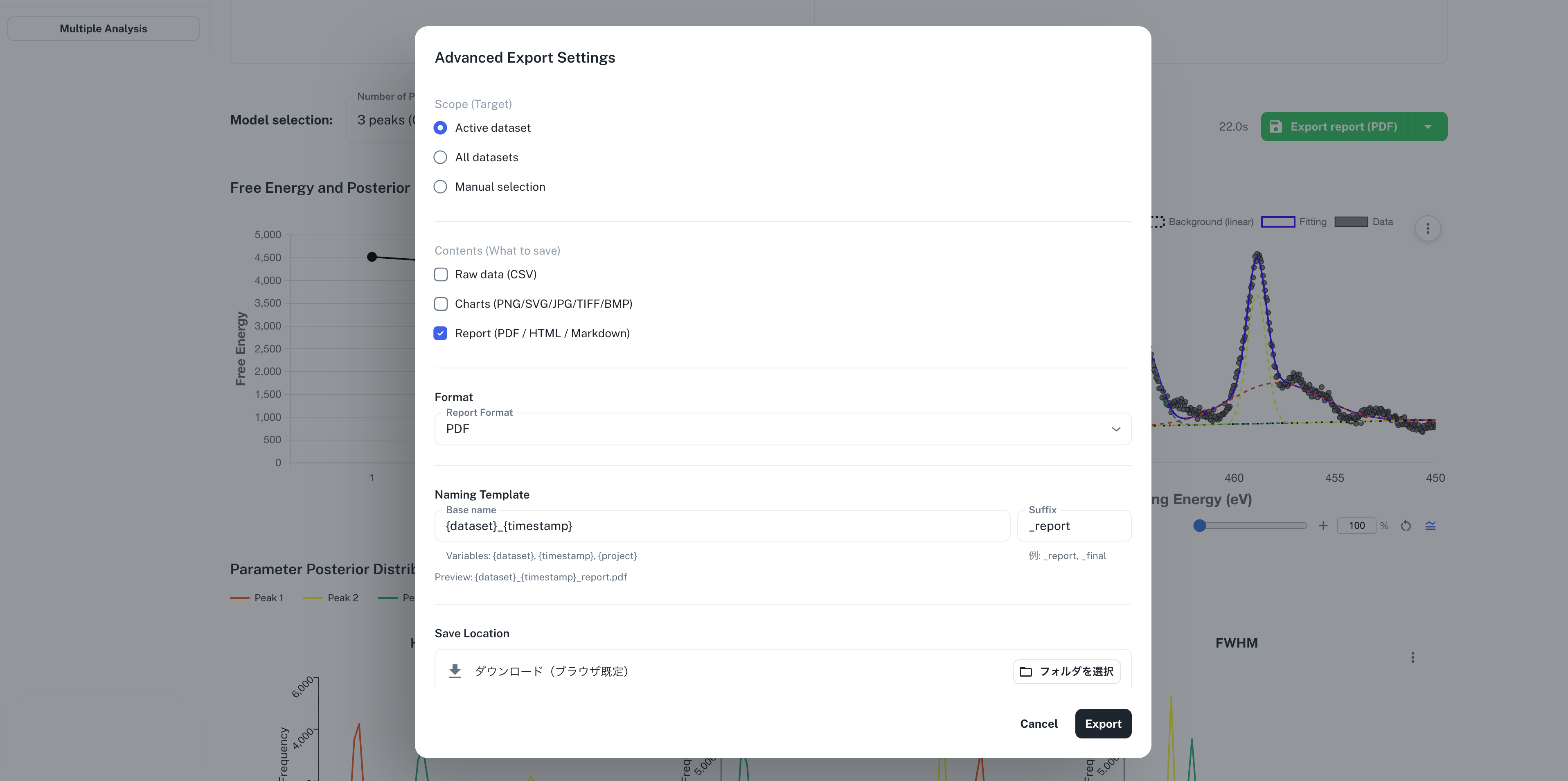
Section	Contents
Scope	Active dataset / All datasets / Manual selection
Contents	CSV / Charts / Report
Format	Report Format: PDF / HTML / Markdown, Chart Format: PNG / SVG / JPG / TIFF / BMP, Chart DPI
Naming	File name template and suffix. {dataset}, {timestamp}, and {project} can be used
Save Location	In the Desktop edition or Chrome / Edge, use Select folder to choose a destination folder.

Report Format offers PDF / HTML / Markdown. Chart Format offers PNG / SVG / JPG / TIFF / BMP. The Chart DPI setting is not applied to some outputs (the batch export of result plots), which may be output at a built-in resolution. In the Desktop edition or Chrome / Edge, use Select folder to choose a destination folder.

11.7 Saving Plot Images

To save plot images in a batch, choose Export images (PNG) from the Export menu. The image ZIP contains the plot images of all models, not only the displayed model, saved in per-model subfolders. Directly under the root, a manifest.json is output recording the selected model, the folder name of the best model, and the list of models.

Each plot on screen can also be saved individually as an image from the menu at its top right. Use this when you want to save the displayed plot as-is.

11.8 Group Analysis Output

In the group analysis results area, the Export split button lets you export the currently displayed data item (Active) and all data items (All datasets) separately.

Export results (CSV) – Active

Saves only the currently displayed data item as a ZIP. A <timestamp>-<data name> folder is created directly under the ZIP root, containing the same root/model folder structure as a single-spectrum Results ZIP.

<timestamp>-<data-name>/
├── summary.json
├── experiment_config.json
├── model_comparison.csv
└── pseudoVoigt-10peaks/
    ├── fit_curve.csv
    ├── parameter_summary.csv
    ├── posterior_samples.csv
    └── statistics.json

Export results (CSV) – All

Saves all analyzed data items in the group together as a ZIP. Folders named after each data item are placed directly under the ZIP root, each containing the same structure as a single-spectrum Results ZIP.

<group-name>/
├── data-a/
│   ├── summary.json
│   └── pseudoVoigt-10peaks/
└── data-b/
    ├── summary.json
    └── pseudoVoigt-10peaks/

Report / images

Export report (PDF) – Active saves only the currently displayed data item as a PDF report. Export report (PDF) – All creates a PDF report for each analyzed data item and bundles them into a single ZIP. Export images (PNG) – Active saves the plot images of the currently displayed data item as a ZIP.

In group analysis exports, the JST timestamp uses the YYYYMMDDHHmmss format without separators (unlike the YYYY-MM-DDTHH-mm-ss format of single-dataset exports).

---

11.9 Examples of Using the Output

• Checking the best model: In model_comparison.csv, find the row where Is_Best_Model is Yes, and refer to fit_curve.csv and parameter_summary.csv in the corresponding subfolder
• Checking the selected model: The row where Is_Selected_Model is Yes is the model that was displayed on screen
• Creating images for reports: Use Export images or the Charts option in Advanced Export
• Reusing the fit results: Load fit_curve.csv into a spreadsheet application or an analysis script
• Inspecting the distributions of estimates: Use posterior_samples.csv or histogram_*.csv
• Saving the analysis conditions: Keep experiment_config.json together with the results folder